Building up to Navier–Stokes, One Term at a Time

The Navier–Stokes equations are key equations that govern everything from the aerodynamics of a wing and the cooling of a microchip to the sprawling circulation of oceans and atmosphere. In Scientific ML, we often embed these equations into loss functions via PINNs, neural operators, or learned closures, treating the PDE as a black-box regularizer (checkout my PINN tutorial here). However, building a model that is physically consistent requires moving beyond from implementation to a mechanical intuition of the fluid itself.

In this post we deconstruct the equations from the ground up, adding one term at a time to see exactly how the physics transforms. We start with the Newton’s second law, apply it to a fluid element, and start relaxing assumptions one at a time with an attempt to show the place of each component in the balance of forces. That way one can understand why a model fails when that term is missing or poorly resolved. Each stage adds a single piece of physics and shows what it does to the same concrete problem: 2D flow past a circular cylinder in a wide channel, uniform inflow from the left.

To achieve a complete physical description, we cannot rely on momentum alone. We should integrate the continuity equation to ensure mass balance, the kinematic requirement that ensures that what flows in must flow out. Next, we must apply constitutive relations to define how the fluid’s internal stresses respond to motion. Without these constraints, the Navier–Stokes equations are underdetermined, meaning it is a system with more unknowns than rules. And finally intial and boundary conditions that tie the flow to the specific geometry in space and time.

Stage 1: Newton’s second law on a fluid element

We start by tracking a small volume of fluid. The second law $F = ma$ is applied per unit volume as:

The left side is the acceleration of a fluid element written in the Eulerian frame. What it means is that we sit at a fixed point in space and watch fluid pass through it rather than moving along with a fluid particle. The combination $\frac{\partial \mathbf{u}}{\partial t} + (\mathbf{u}\cdot\nabla)\mathbf{u}$ is the material derivative $\frac{D\mathbf{u}}{Dt}$: the first term is the local rate of change at that fixed point; the second corrects for the fact that the element is also moving into regions with different velocity. That second term, $(\mathbf{u}\cdot\nabla)\mathbf{u}$, is the nonlinear advective term. That vector is the one responsible for essentially everything interesting in fluid dynamics.

Conditions for this stage:

• Initial Condition: $\mathbf{u}(\mathbf{x}, 0) = \mathbf{U}_\infty$
• Boundary Conditions: $\mathbf{u} = \mathbf{U}_\infty$ on all boundaries.

With no forces on the right ($f=0$), the fluid just flows on a straight line, so the obstacle is invisible for the fluid. We get a uniform flow.

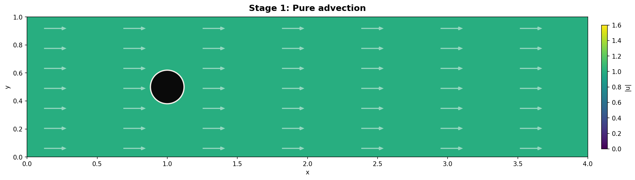
This is the simplest baseline we start building on. But something is missing.

Stage 2: Add Pressure and Kinematic Constraints

Fluid at the front of the cylinder can not keep going forward as cylinder is a boundary obstacle that is pushing the fluid sideways. More specifically, it creates a pressure gradient, a scalar field that pushes along its negative gradient equally in all directions:

This is called the Euler equation that governs flow of an ideal fluid with no internal friction. To close the system as we have an extra variable now, we also need mass conservation, or conintuity, (incompressible for now) equation:

Conditions for this stage:

• Initial Condition: $\mathbf{u}(\mathbf{x}, 0) = \text{Potential Flow Solution}$
• Inflow/Outflow: $\mathbf{u} = \mathbf{U}_\infty$
• Cylinder Boundary: $\mathbf{u} \cdot \mathbf{n} = 0$ (No-penetration; fluid slides freely)

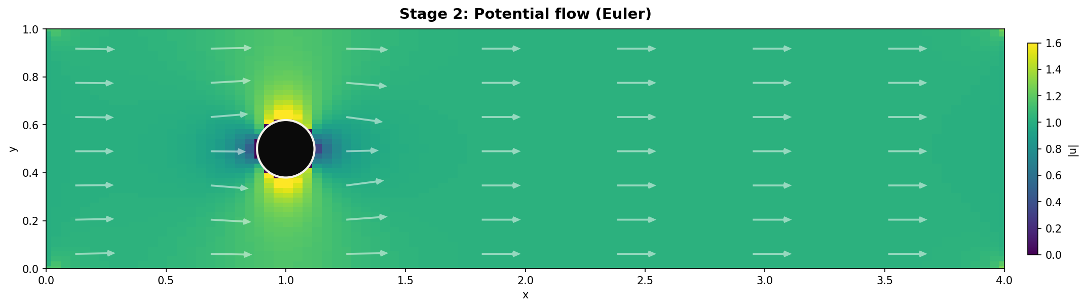
Now the fluid knows the cylinder is there and shapes around it by accelerating over the top and bottom (Bernoulli: faster flow, lower pressure), and recovers on the far side. The picture is perfectly symmetric as integrating pressure around the cylinder gives zero drag. An inviscid fluid (fluid without viscosity) exerts no drag on an obstacle, which we know is wrong for real fluids.

This is actually one of the rare cases in fluid dynamics where we can write down the exact answer. Since there’s no viscosity, vorticity is never created, so the flow stays irrotational: $\nabla \times \mathbf{u} = 0$. That means we can write $\mathbf{u} = \nabla \phi$ for a velocity potential $\phi$, and the continuity equation $\nabla \cdot \mathbf{u} = 0$ collapses to Laplace’s equation:

For a cylinder of radius $R$ centered at the origin with uniform inflow $U_\infty$ from the left, the solution in polar coordinates is:

The first term is the uniform stream; the second is a dipole that enforces the no-penetration condition at the cylinder wall. Taking the gradient gives the velocity field:

You can verify: at $r = R$, the radial component $u_r = 0$ (nothing goes through the wall), while the tangential component $u_\theta = -2U_\infty \sin\theta$ (the fluid slides freely along the surface as there is no viscosity, no no-slip). The speed peaks at the top and bottom of the cylinder ($\theta = \pm\pi/2$) at twice the free-stream value.

Pressure follows from Bernoulli’s equation along any streamline:

Integrating this pressure over the cylinder surface gives exactly zero net force in every direction, so called d’Alembert’s paradox. The high pressure at the front stagnation point is perfectly mirrored at the rear. This is the analytical proof that inviscid flow can’t produce drag, so something is still missing.

Stage 3: Add Viscosity and Constitutive Relations

Real fluids resist shear, so called internal traction: neighboring layers moving at different speeds drag on each other. Model that drag as proportional to velocity gradients (Newtonian fluid, one free parameter $\mu$), and the momentum equation gains a Laplacian term:

This is the incompressible Navier–Stokes system which is closed as there are four equations (three components of momentum plus divergence-free constraint) and four unknowns ($\mathbf{u}$ and $p$).

Conditions for this stage:

• Initial Condition: $\mathbf{u}(\mathbf{x}, 0) = \mathbf{u}_{initial}$
• Cylinder Boundary: $\mathbf{u} = 0$ (The no-slip condition)

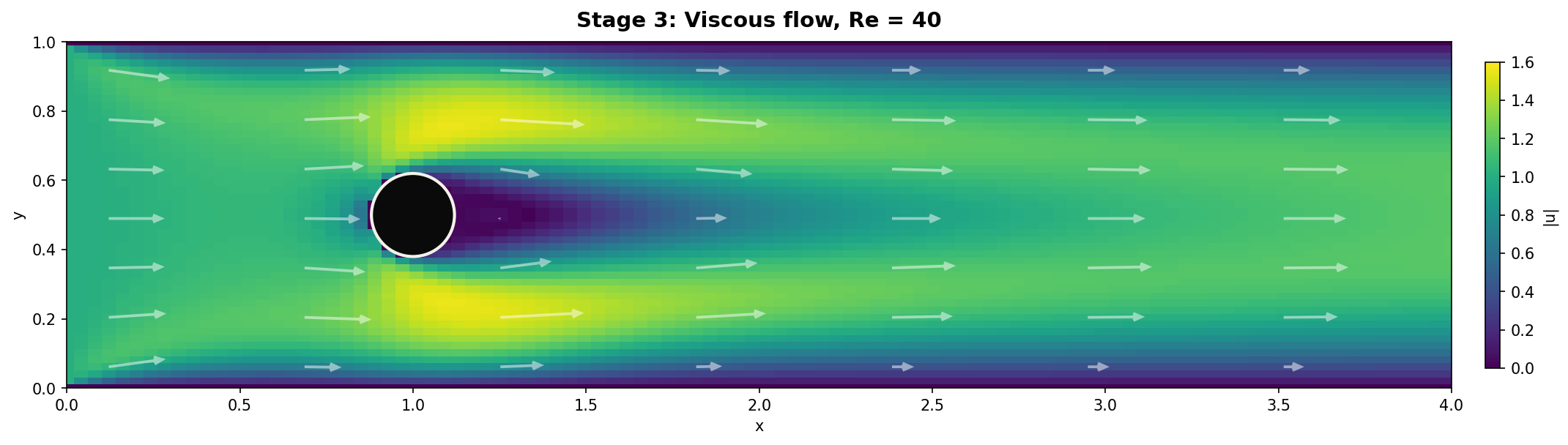
Viscosity does two things. First, it enforces no-slip at solid boundaries, so the fluid in direct contact with the cylinder has the cylinder’s velocity, which is zero. This creates a boundary layer where velocity ramps up from 0 to the free-stream value. Second, it dissipates kinetic energy: moving fluid in the wake is irrecoverably lost, which is what drag actually is.

At Reynolds number, in a sense a measure of tubulence, $Re = UL/\mu \approx 40$, a standing pair of recirculation vortices appears behind the cylinder. The front-back symmetry is broken, so pressure recovers less on the downstream side. The drag force is not not zero and causes that asymmetry.

Stage 4: Same equations, higher Re

We drop viscosity further, so $Re \approx 150$. The equations and boundary conditions are identical to Stage 3, only the coefficient $\mu$ changes.

Conditions for this stage:

• Boundary Conditions: Identical to Stage 3 (no-slip).

The behavior changes qualitatively: the wake becomes unsteady, and vortices begin to shed alternately (vortex shedding). This is the nonlinear term asserting itself, demonstrating that the system does not scale linearly.

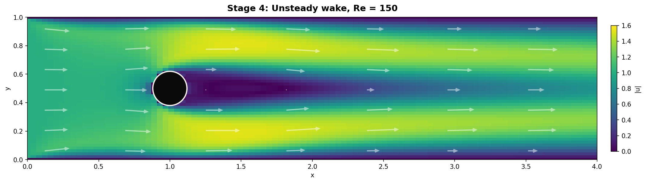
Nothing new was added to the equations. This is purely the nonlinear term $(\mathbf{u}\cdot\nabla)\mathbf{u}$ asserting itself: it couples scales, it destabilizes steady solutions, and at high enough Reynolds numbers it produces the turbulence. In a sense, this nonlinear model is not scaling predictibally anymore, as doubling the inflow velocity doesn’t double the answer past a threshold, it changes the type of the flow.

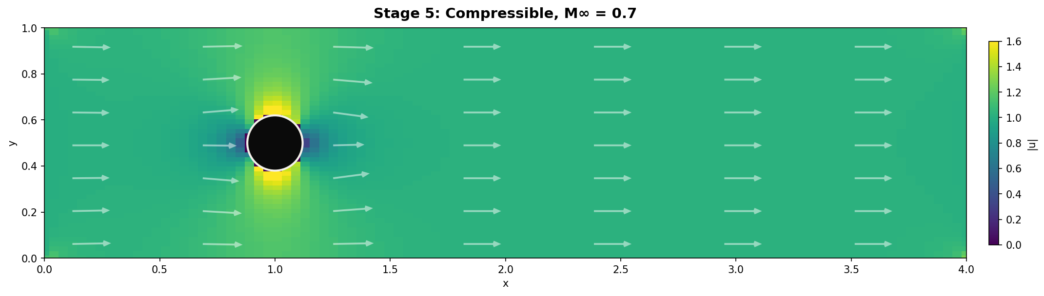
Stage 5: Relax incompressibility

Finally we allow density to vary requiring a full set of conservation laws and an equation of state: \(\frac{\partial \rho}{\partial t} + \nabla \cdot (\rho \mathbf{u}) = 0\)

Conditions for this stage:

• Initial Conditions: Specified $\rho, \mathbf{u}, T$ fields.
• Boundary Conditions: No-slip and no-penetration, plus thermal conditions (e.g., adiabatic or isothermal walls).

Now $\rho$ is a field with its own evolution equation (continuity). We need an equation of state tying pressure to density and temperature, and strictly we’d add an energy equation too. The viscous stress generalizes to a tensor $\boldsymbol{\tau}$ that accounts for bulk expansion.

The system changes from elliptic in pressure to hyperbolic. Disturbances propagate at the speed of sound rather than infinitely fast. Shocks and sound waves emerge, phenomena that simply do not exist in the incompressible world.

For flows well below the speed of sound like water through a pipe, air over a slow object density changes are negligible ($\mathcal{O}(M^2)$ where $M$ is the Mach number) and the incompressible equations are exact enough. For transonic or supersonic flows, you have no choice but to use the full compressible system.

Why this matters if you’re training models

If you are building a PINN or a neural operator, every term we added is a physical commitment your network must respect. If your model predicts zero drag, it hasn’t captured viscosity (Stage 2). If conservation is violated, your divergence-free constraint is failing. The Navier–Stokes system isn’t a black box; it’s a sequence of doors to physical phenomena. The better you understand which door you’re walking through, the better you’ll know where to look when your model breaks.

If you want to play with the cylinder problem yourself, toggle viscosity and compressibility below to see the stages in real time.

Citation

If you find this work useful, please cite:

@article{levonyan2026navierstokes,
  title={Building up to Navier–Stokes, One Term at a Time},
  author={Levonyan, Karine},
  year={2026},
  url={https://karinelevonyan.github.io/blog/2026/navier-stokes-one-term-at-a-time/}
}