Internal Biases in the Visual Latent Space: A Comparative Empirical Study
In natural language processing, the vector arithmetic $\text{King} - \text{Man} + \text{Woman} \approx \text{Queen}$, though not precise, but became a foundational proof that language models capture structured semantic relationships. As if the model learned to associate the direction of a “gender” in this example to the difference between two latent vectors. Can vision models do the same? Do visual encoders span a latent space structured well enough to compute analogies through linear transformations, with $z_D \approx z_C + (z_B - z_A)$?
This post is an attempt to analyze the vision embeddings latent spaces. One could hypothesis that that answer depends entirely on the worldview baked into each encoder. Model architecture and optimization objective push a model toward a particular geometry, and that geometry is the bias we want to measure. This post compares four such worldviews: CLIP, DINOv2, Supervised ViT, and Visual Autoregressive (VAR) models. It then runs seven controlled experiments to map where each model succeeds and where it fails.
Every figure below comes from experiments.py. The empirical numbers come from those runs.
Four Visual Worldviews
Before any plots, it helps to fix a vocabulary for the way these models behave when we start doing arithmetic on their embedding vectors. So we define four different embedding personalities.
CLIP: the Semantic Librarian
CLIP uses a coupled encoder, one for text and one for images, trained on hundreds of millions of matched image-text pairs. The training objective is a contrastive loss that pulls true pairs together in cosine space and pushes mismatched pairs apart. Because the image encoder is anchored to natural language, it learns to discard local pixel dynamics in favor of global linguistic concepts. In short, images appearing in a similar text captions are closer to each other.
DINOv2: the Structural Architect
DINOv2 uses self-distillation with no human labels. A student network learns to match a teacher’s output across different crops of the same image. The loss has both an image-level term and a patch-level term. The patch-level objective forces the model to learn continuous fields of geometry, depth, and structural boundary. It treats images as networks of interconnected local components, so it is able to differentiate between physica geometry and object parts.
Supervised ViT: the Categorical Specialist
A standard Vision Transformer trained with cross-entropy against ImageNet’s 1,000 classes. Decision boundaries between classes define the space directly. Hence, features that do not help separate those classes get compressed away.
VAR: the Impressionist
Unlike the continuous encoders above, VAR operates over quantized visual tokens drawn from a discrete codebook (VQ codebook). It models images hierarchically, predicting token maps from coarse scales like $1{\times}1$ and $2{\times}2$ down to fine scales like $16{\times}16$. The analogy operation is no longer vector arithmetic. It becomes token substitution, where we swap one codebook index for another. It prioritizes colors and textures over high-level.
A note on the implementation. The VAR results below use a stand-in for a real VQ-VAE codebook. We run k-means over raw 14×14 RGB pixel patches. This is not a trained VAR codebook, but it preserves the properties we care about: discrete tokens, hierarchical pooling, and substitution instead of addition.
We apply edge arithmetic to simplistic edge cases to reveal biases of these models.
Cluster Geometry: How Each Model Sees the World
We embed identical CIFAR-10 images with each continuous backbone and project to 2D with UMAP. For VAR we overlay the discrete-token histogram instead.
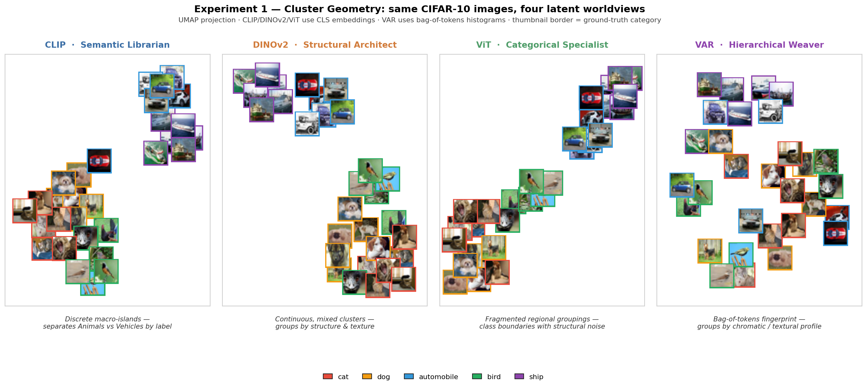
- CLIP yields discrete macro-islands with sharp separation between major semantic categories such as animals versus vehicles. It groups by language label regardless of background or texture.
- DINOv2 produces a continuous, uniformly distributed space with mixed semantic clusters. It links objects that share raw geometric profiles, edge alignments, or material texture rather than abstract labels.
- Supervised ViT sits in between, with fragmented clusters and loose regional groupings. The class boundaries are strong, but the structural noise is visible.
- VAR lives in token space, so we plot the bag-of-tokens histogram instead. Each image becomes a chromatic and textural fingerprint over the codebook. There is no UMAP here because there is no continuous manifold to embed.
Analogy Arithmetic: Does the Latent Space Compose?
The cleanest test of compositional structure is a controlled four-point analogy. We define it as follows.
\[\text{Yellow Circle}\ (A) \rightarrow \text{Blue Circle}\ (B) \;::\; \text{Yellow Square}\ (C) \rightarrow \text{?}\ (D)\]If the encoder has truly separated color from shape, then $z_C + (z_B - z_A)$ should land near the blue square. We measure cosine similarity to the true target and verify the result with nearest-neighbor retrieval. For VAR, arithmetic gives way to token substitution. We learn the $A \rightarrow B$ swap rule from the first pair, then apply it to $C$.
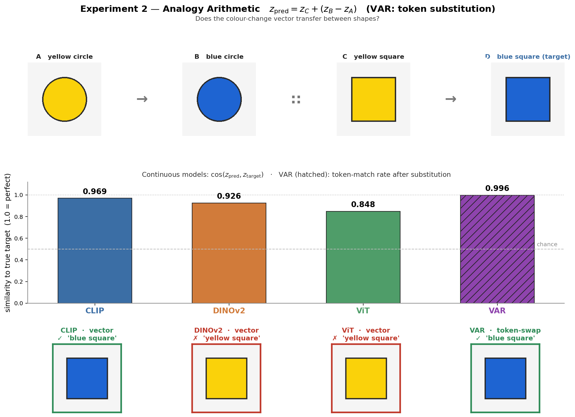
- CLIP safely identifies the blue square as its absolute nearest neighbor. Color and shape act as independent, language-grade abstractions that compose cleanly.
- DINOv2 fails retrieval and snaps back to a yellow square. Its representation entangles color with the patch-level structural signature, so the linear delta corrupts the boundary instead of swapping the fill.
- ViT also fails and returns a yellow square. Its class-discriminative features do not factor color and shape into orthogonal directions.
- VAR succeeds symbolically. The learned token-swap rule, such as codebook index 3 mapping to index 0 wherever it appears in $C$, reconstructs the blue square at a 99.6% token-match rate.
Residual Heatmaps
For this experiment we would like to understand where does the difference vector live in the embedding space. For each patch of image $A$ versus image $B$, we measure the magnitude of the local change in the patch embeddings. For VAR we use centroid-cosine distances between corresponding token centroids.
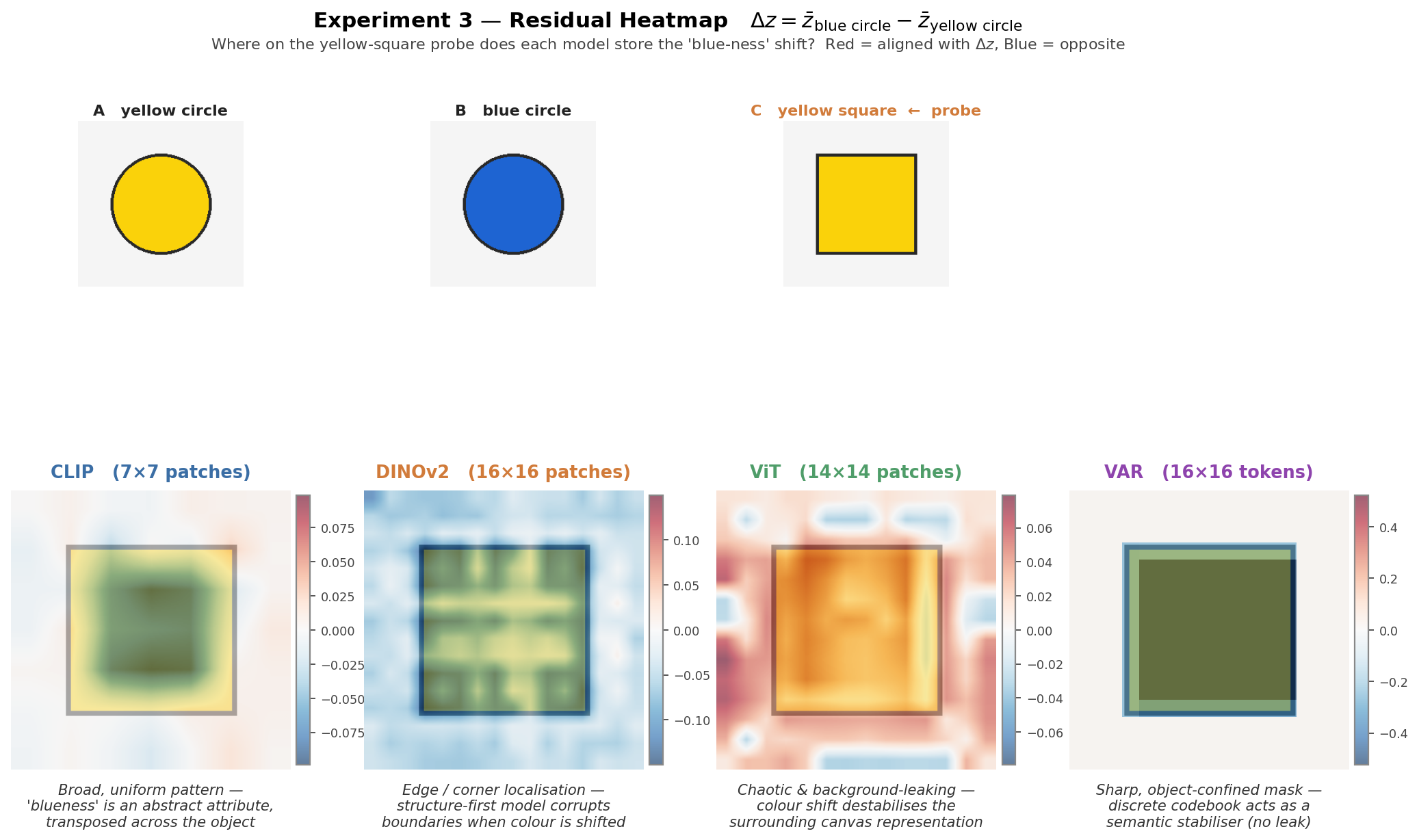
- CLIP shows broad, uniform heat across the object. Blue-ness sits as a global, transposable attribute, which is exactly what let the analogy in section III succeed.
- DINOv2 shows intense localization along edges and corners. The model encodes color through its structural boundary description, so the analogy delta corrupts the silhouette.
- ViT shows a chaotic heatmap that leaks heavily into the background canvas. The encoder cannot isolate the object from its surroundings.
- VAR shows a sharp, object-confined response. The discrete codebook acts as a semantic stabilizer and refuses to put heat in places where no codebook entry changed.
Spatial Sensitivity
With this test we would like to test spatial. We take identical objects (a cat, an automobile, and a bird) and translate them into the four quadrants of an empty square. We then compute the mean pairwise cosine distance across all position pairs. We would like to see an almost diagonally dominated variogram: a high distance means the model tracks position, a low distance means the model is invariant to it.
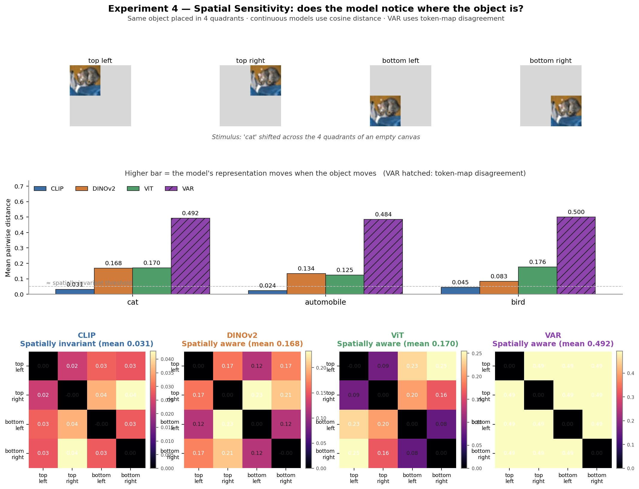
| Model | Cat | Auto | Bird | Characterization |
|---|---|---|---|---|
| CLIP | 0.031 | 0.024 | 0.045 | Spatially invariant |
| DINOv2 | 0.170 | 0.134 | 0.084 | Spatially aware |
| ViT | 0.171 | 0.125 | 0.177 | Spatially aware |
| VAR | n/a | n/a | n/a | Highly position-bound (large token-map disagreement) |
CLIP’s blindness is structural. Language-supervised contrastive training rewards the encoder for ignoring spatial nuisance. A cat in the top left and a cat in the bottom right serve identical text captions, so they collapse to the same point.
DINOv2 and ViT keep position information because their patch-level losses (DINOv2) or grid-bound classification features (ViT) need it. VAR shows the highest spatial sensitivity of all the models tested. Changing position changes which codebook indices appear at which tile, and the token maps disagree almost everywhere.
This is the first place we see a clear dilemma. The same property is a feature in one task and a bug in another. CLIP’s invariance helps it retrieve a cat regardless of pose. DINOv2’s awareness helps it segment that same cat from its surroundings.
Token Substitution and the Global Consistency Trap
VAR replaces the continuous arithmetic of section III with discrete token substitution. Rather than walking 0.5 units in a blue direction, the model swaps codebook index $i$ for index $j$. We can ask the same analogy question, yellow to blue applied to a yellow square, and watch the swap propagate.
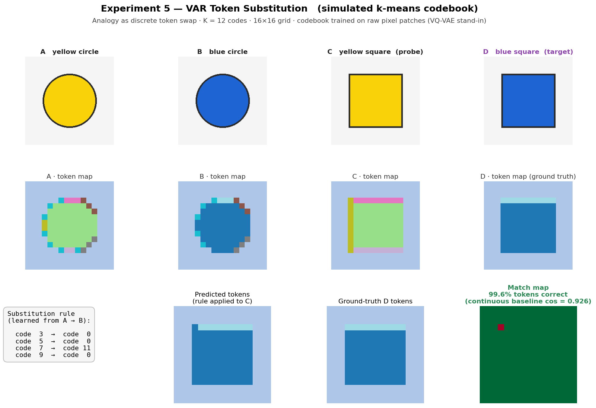
The discrete codebook prevents the leaky-background failure from section IV. Substitutions can only land on valid codebook entries, so the model cannot wander off into a corrupted region of the manifold. Discreteness brings its own failure mode, though, and it becomes visible once we look at VAR’s hierarchical structure.
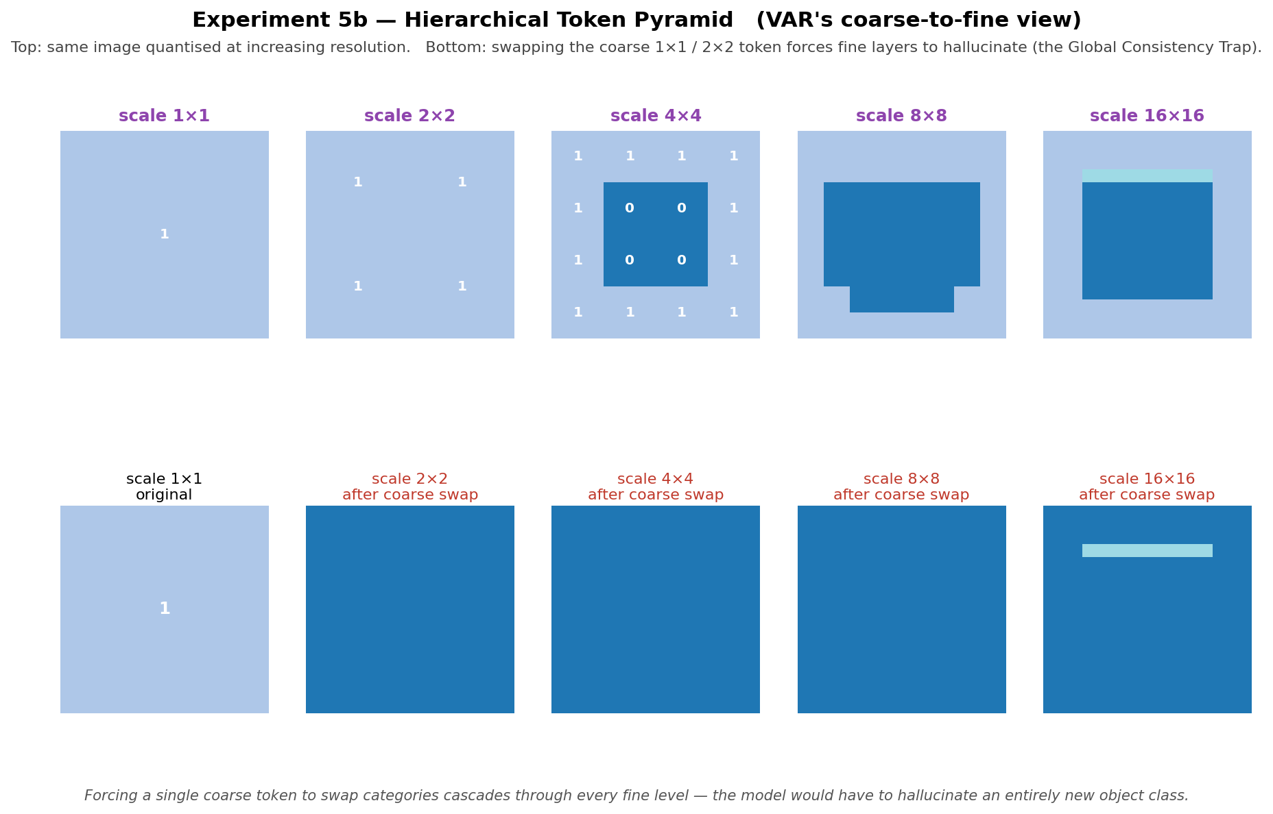
The pyramid shows the image quantized at $1{\times}1$, $2{\times}2$, $4{\times}4$, $8{\times}8$, and $16{\times}16$ scales. A swap at the coarsest level forces every fine-scale token to remain consistent with the new identity. If the codebook has not learned to separate size or context from object identity, that consistency requirement can hallucinate an entirely new object class. We call this the Global Consistency Trap. Forcing a blue token at the coarse scale can turn a transparent square into a glass bottle, simply because that is the closest plausible assembly of fine tokens.
Counting Problem
Finally, we test foris these spaces understand discrete numbers?
\[1\ \text{red circle}\ (A) \rightarrow 3\ \text{red circles}\ (B) \;::\; 1\ \text{blue circle}\ (C) \rightarrow \text{?}\]A perfect encoder should predict three blue circles.
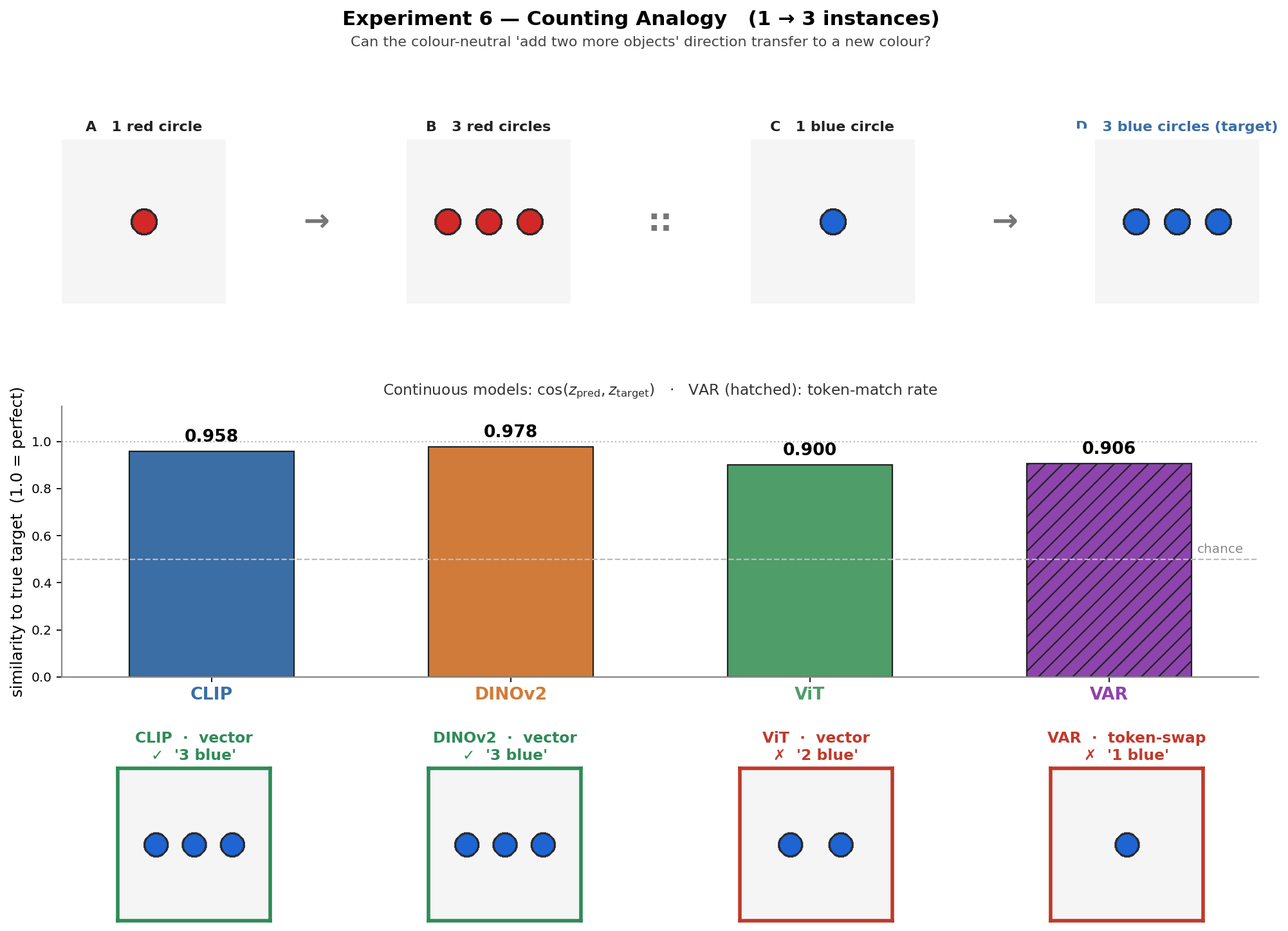
The cosine numbers look uniformly high. CLIP scores 0.958, DINOv2 scores 0.978, ViT scores 0.900, and VAR scores 0.906. The nearest-neighbor retrievals tell a different story. CLIP and DINOv2 retrieve the correct three-blue-circles target. ViT retrieves only two blue circles. The discrete VAR system collapses back to a single blue circle. With no explicit notion of cardinality in the codebook, the operation of adding two more instances cannot be expressed as a token swap. Continuous spaces approximate counting. Discrete token spaces, without a counting prior, do not.
This is the first experiment where CLIP and DINOv2 outperform VAR, and the reason is structural. VAR’s strength is substitution, and substitution is the wrong primitive for instance multiplication.
Lighting: Is “Night” a Transferable Concept?
Can a model extract “night” as a property independent of what is being lit?
\[\text{city·day}\ (A) \rightarrow \text{city·night}\ (B) \;::\; \text{forest·day}\ (C) \rightarrow \text{?}\]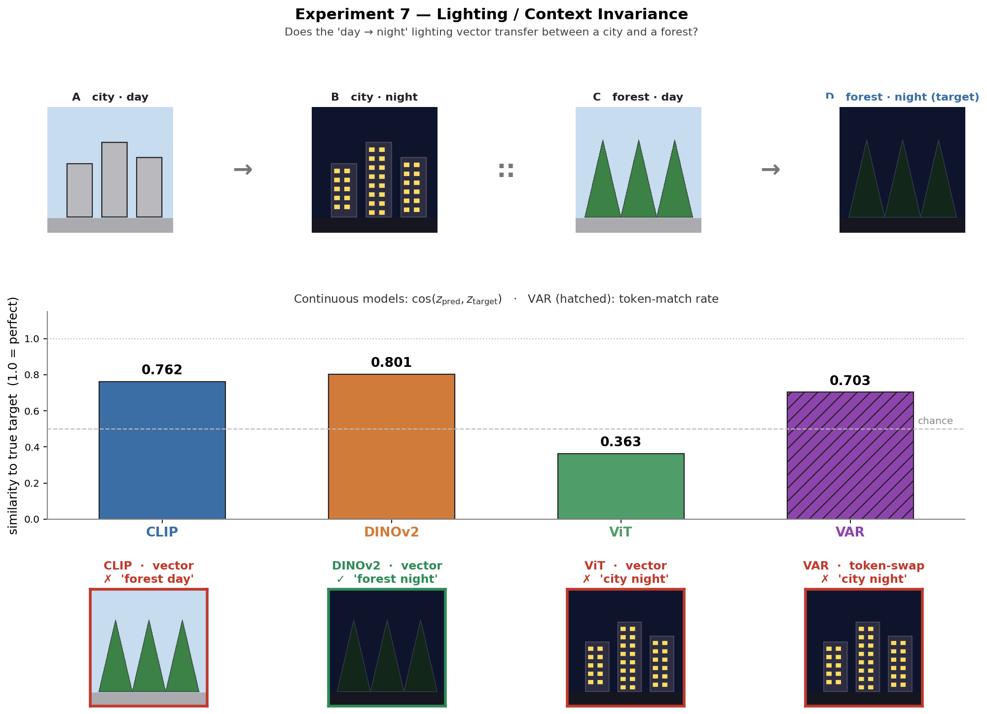
Only DINOv2 retrieves the correct forest-at-night target, with a score of 0.801. Its patch-level training has separated ambient illumination from object identity, so the day-to-night vector lifts cleanly from one scene type to another. CLIP scores 0.762 but retrieves a daytime forest, because lighting is partially entangled with the forest concept in its caption-aligned space. ViT collapses to 0.363, well below the chance line for day-night and scene type, and snaps back to a city. Its class-discriminative features cannot separate scene type from lighting. VAR scores 0.703 and retrieves a city night scene. The token substitution it learned on city pixels does not generalize to the forest’s geometry.
This experiment mirrors section VII. Counting punished the discrete model. Context invariance rewards the patch-level structural decomposition that DINOv2 learns natively.
Experiments Model
The seven experiments above all follow the same computational flow. To replicate or extend the study:
- Data pipeline. Standardize inputs to $224 \times 224$. Construct controlled triplets $(A, B, C)$ where exactly one attribute changes between $A$ and $B$, and that attribute is the one we want to transfer onto $C$.
- Feature extraction. Load weights from Hugging Face:
openai/clip-vit-base-patch32,facebook/dinov2-base, andgoogle/vit-base-patch16-224. Pull the[CLS]embedding for global tests, and pull patch embeddings for the residual heatmaps. - Normalization. L2-normalize every vector before any cosine work, so that $\hat z = z / |z|_2$. Cosine similarity is only meaningful on the unit hypersphere.
- Analogy arithmetic. Compute $\Delta z = \hat z_B - \hat z_A$, then $z_\text{pred} = \hat z_C + \Delta z$, re-normalize the result, and verify by k-nearest-neighbor retrieval against an evaluation pool.
- Spatial drift. Slide a single object across the four quadrants of a blank canvas, then compute the full $4 \times 4$ pairwise cosine distance matrix.
- Attribution heatmaps. Project $|\Delta z_\text{patch}|$ back onto the spatial grid.
- VAR stand-in. When a real codebook is unavailable, k-means over raw 14×14 pixel patches plus mode-pooling at coarser scales reproduces enough of the discrete and hierarchical structure to support qualitative claims.
Discussion
No single encoder wins across every test. While CLIP handles compositional and counting tasks well, DINOv2 wins on structural and lighting tasks. ViT loses most analogy tasks but tracks spatial position cleanly. VAR stabilizes attribute edits, cannot count, and stays rigidly tied to position.
Each model’s bias is the geometry of its training objective made visible. Contrastive language alignment produces global, linguistic, position-invariant features. Patch-level self-distillation produces local, structural, position-aware features. Cross-entropy supervision carves class boundaries at the cost of compositional smoothness. Discrete autoregressive prediction enforces hierarchical token coherence at the cost of cardinality and translation.
The right encoder for a given job is the one whose bias matches that job. Finding a cat anywhere in an image plays to CLIP’s strengths, while segmenting that same cat from the wall is a DINOv2 task. The arithmetic operation we have been running serves as a probe of the encoder, not a property of vision itself. The lesson from word embeddings, that the geometry encodes the training signal, carries directly into vision. Vision adds one wrinkle: it offers many more axes along which a model can be entangled or factored, including color, shape, position, count, and illumination.
References
- Oquab, M., et al. (2023). DINOv2: Learning Robust Visual Features without Supervision. arXiv:2304.07193.
- Radford, A., et al. (2021). Learning Transferable Visual Models From Natural Language Supervision. ICML.
- Reed, S. E., et al. (2015). Deep Visual Analogy-Making. NeurIPS.
- Tian, K., et al. (2024). Visual Autoregressive Modeling: Scalable Image Generation via Next-Scale Prediction. arXiv:2404.02905.
- Yuksekgonul, M., et al. (2022). When and Why Vision-Language Models Behave like Bags-of-Words. ICLR Blog Track.
Citation
If you find this work useful, please cite:
@article{levonyan2026visualbias,
  title={Internal Biases in the Visual Latent Space: A Comparative Empirical Study},
  author={Levonyan, Karine},
  year={2026},
  url={https://karinelevonyan.github.io/blog/2026/internal-biases-visual-latent-space/}
}