Why the Drift Field Finds the Right Distribution for SPD Kernels: Proof
Building on Deng et al. (2026) and Ziming Liu’s physical interpretation
One Forward Pass Is All You Need: Is Equillibrium Unique?
Current generative models carry significant computational cost at inference time. Diffusion models require hundreds of sequential denoising step which is slow. Flow matching are more efficient with good ODE sovlers, but still requires multiple forward passes. GANs demand adversarial optimization with stability issues. In each case the iterative structure, whether at inference or during training, trades off between quality and efficiency.
Deng et al. (2026) propose a fundamentally different approach. Their drifting models train a single-pass generator whose output distribution evolves during training via a drift field $\mathbf{V}_{p,q}$, then produce samples in one forward evaluation at test time. The drift field acts as a force: generated samples are attracted toward data points and repelled from one another, analogous to a system of charged particles relaxing toward electrostatic equilibrium. When the generated distribution $q$ matches the data distribution $p$, the net force vanishes and the system reaches a fixed point.
This electrostatic analogy is not just illustration, In fact, as Liu (2026) observed, the paper’s kernel $k(r) = \exp(-r/\tau)$ corresponds to a Yukawa potential, placing the framework within classical field theory. The screening length $\tau$ determines the interaction range, and the equilibrium condition $\mathbf{V} = 0$ is a statement of global force balance.
The central theoretical question is whether this equilibrium is unique. The original paper establishes one direction, that $q = p$ implies $\mathbf{V} = 0$, but leaves the converse as an open problem. Without it, the training objective could admit spurious equilibria: configurations where the drift field vanishes identically but $q \neq p$. This post attemprs to resolve that question.
The Result
Deng et al. (2026) introduce Drifting Models, a generative paradigm where a vector field $\mathbf{V}_{p,q}$ pushes generated samples $x \sim q$ toward the data distribution $p$ during training, yielding one-step inference. They prove that $q = p$ implies $\mathbf{V} = 0$ (equilibrium), but leave the converse open (Section 6, Appendix C.1):
“The converse implication, i.e., $\mathbf{V}_{p,q} = 0 \Rightarrow q = p$, is false in general for arbitrary choices of V.”
Without the converse, a kernel could admit spurious equilibria, configurations where $\mathbf{V} = 0$ but $q \neq p$. That means that training would converge to the wrong distribution.
This post attempts to close that gap. For any strictly positive definite kernel, including the Laplace kernel the paper uses, we prove via Bochner’s theorem that $\mathbf{V} = 0$ implies $q = p$. The proof also identifies exactly which kernels preserve this guarantee and which do not, and it yields a principled rule for choosing the temperature parameter $\tau$.
Ziming Liu’s post provided the physical intuition that guided this analysis. His interpretation of generated samples as negatively charged particles attracted to positively charged data points, interacting through a Yukawa potential $k(r) = e^{-r/\tau}$, reframes the convergence question in the language of screened electrostatics. From that viewpoint, the converse question becomes: can a Yukawa charge configuration be in perfect force balance without every negative charge sitting on top of a positive one? The answer, via Bochner’s theorem, is no.
Setup and Notation
The drift field from the paper (Eq. 8–9 of Deng et al.) is:
\[\mathbf{V}_{p,q}(x) = \mathbb{E}_{y^+ \sim p,\, y^- \sim q}\!\left[\tilde{k}(x, y^+)\,\tilde{k}(x, y^-)\,(y^+ - y^-)\right] \tag{1}\]where $\tilde{k}$ denotes the batch-normalized kernel. The paper uses:
\[k(x, y) = \exp\!\left(-\frac{\|x - y\|}{\tau}\right) \tag{2}\]This is the Laplace kernel, or, in Liu’s physical language, a Yukawa potential with screening length $\tau$.
The paper proves the forward direction (their Proposition 3.1):
\[q = p \;\Rightarrow\; \mathbf{V}_{p,q}(x) = 0 \quad \forall x \tag{3}\]This follows immediately from anti-symmetry: swapping $p \leftrightarrow q$ negates $\mathbf{V}$, so when $p = q$ we get $\mathbf{V} = -\mathbf{V} = 0$.
The converse, whether $\mathbf{V} = 0$ forces $q = p$, is what we prove below.
Which Kernels Are SPD?
A translation-invariant kernel $k(x-y)$ is strictly positive definite (SPD) if and only if its Fourier transform $\hat{k}(\omega) > 0$ for all $\omega$. Equivalently, the kernel has no blind spots in frequency space. This is Bochner’s classical characterization (1933). A kernel that is SPD is also characteristic: the kernel mean embedding $\nu \mapsto \int k(\cdot, y)\,d\nu(y)$ is one-to-one on probability measures, meaning no two distinct distributions can produce the same embedding (Sriperumbudur et al., 2010).
The paper’s Laplace kernel $k(x-y) = e^{-|x-y|/\tau}$ is SPD: its Fourier transform is the Cauchy distribution
\[\hat{k}(\omega) = \frac{c_d \,\tau^d}{(1 + \tau^2\|\omega\|^2)^{(d+1)/2}} > 0 \quad \forall\, \omega \tag{4}\]which is strictly positive everywhere. The Gaussian kernel ($\hat{k}$ = Gaussian) and Matérn family ($\hat{k}$ = generalized Cauchy) are also SPD by the same test.
Closing the Converse
Theorem. Let $k(x-y) > 0$ be a strictly positive definite translation-invariant kernel (Laplace, Gaussian, or Matérn) with $k(z) \to 0$ as $\lvert z \rvert \to \infty$. If $p$ and $q$ are compactly supported probability distributions with $\mathbf{V}_{p,q}(x) = 0$ for all $x$, then $p = q$.
The proof in linear algebra terms. We can think of the kernel operator $K_\nu(x) = \int k(x-y)\,d\nu(y)$ as a matrix $A$ acting on distributions. For an SPD kernel, $A$ has all positive eigenvalues (Bochner) and therefore trivial null space: $A\mathbf{v} = 0$, implies $\mathbf{v} = 0$. This is the characteristic kernel property (Sriperumbudur et al., 2010). If the drift condition gave us $K_p = K_q$ directly, we’d be done in one line by null-space injectivity. But the drift gives us something weaker, i.e. equal ratios $M_p/K_p = M_q/K_q$, which is a bilinear constraint, not a linear one. The work of the proof is converting this ratio equality into the linear equation $\Phi_p = \Phi_q$ that the null-space argument can close.
Physical intuition. In Liu’s electrostatic framework, $\mathbf{V} = 0$ means every negative charge (generated sample) is in perfect force balance, i.e. the attraction from positive charges (data) exactly cancels the repulsion from other negatives, at every point in space. The proof asks: can such a perfect balance exist when the charges don’t overlap? We show the answer is no, by “listening” to the force balance from far away. At large distance, the Yukawa potential simplifies to an exponential tilt, and the balance condition becomes a constraint on the moment generating functions of $p$ and $q$. The normalization constraint (both are probability distributions with total mass 1) then forces $p = q$.
Proof. Write $\delta = p - q$.
Step 1: Equal mean-shift fields. Since $k > 0$, the normalization in $\mathbf{V}$ is well-defined, and $\mathbf{V} = 0$ if and only if the unnormalized drift vanishes. Define the kernel-weighted moments:
\[K_\nu(x) = \int k(x-y)\,d\nu(y), \qquad M_\nu(x) = \int k(x-y)\,y\,d\nu(y)\]Expanding $(y^+ - y^-)$ in the drift integral and factorizing (the two kernel terms depend on separate integration variables), $\mathbf{V} = 0$ gives:
\[M_p(x)\, K_q(x) = M_q(x)\, K_p(x) \quad \forall x \tag{5}\]Since $K_p(x), K_q(x) > 0$ everywhere (because $k > 0$ and $p, q$ are probability measures), divide:
\[\frac{M_p(x)}{K_p(x)} = \frac{M_q(x)}{K_q(x)} \quad \forall x \tag{6}\]Each side is the kernel-weighted average position, the mean-shift vector. Physically: the “center of attraction” that a test charge at $x$ feels from $p$ is the same as from $q$, everywhere. In null-space language: the ratio of the first-moment embedding to the zeroth-moment embedding is the same for both distributions. But this is weaker than $K_p = K_q$, so we cannot apply injectivity directly.
If $K_\delta(x) = 0$ for all $x$, the kernel embedding of $\delta$ is the zero vector, then $\delta = 0$ by trivial null space (Sriperumbudur et al., 2010). Done. Otherwise, proceed.
Step 2: Listen from far away. For compactly supported measures, take $x$ far from the data: $\lvert x \rvert \to \infty$ in direction $\hat{u} = x/\lvert x \rvert$. The kernel simplifies — the Yukawa potential at long range becomes a pure exponential tilt:
\[k(x - y) \;\approx\; e^{-\lvert x \rvert/\tau} \cdot e^{(\hat{u} \cdot y)/\tau}\]The prefactor $e^{-\lvert x \rvert/\tau}$ cancels in the ratio (6). What survives is the exponentially tilted mean:
\[\frac{\int y_j\, e^{(\hat{u}\cdot y)/\tau}\, dp(y)}{\int e^{(\hat{u}\cdot y)/\tau}\, dp(y)} = \frac{\int y_j\, e^{(\hat{u}\cdot y)/\tau}\, dq(y)}{\int e^{(\hat{u}\cdot y)/\tau}\, dq(y)} \tag{7}\]Define the moment generating function $\Phi_\nu(s) := \int e^{s \cdot y}\,d\nu(y)$. Each ratio in (7) is $\frac{\partial}{\partial s_j}\log\Phi_\nu(s)$ — the log-MGF gradient. So (7) says:
\[\nabla_s \log\Phi_p(s) = \nabla_s \log\Phi_q(s) \tag{8}\]on the sphere $\lvert s \rvert = 1/\tau$. (For Gaussian kernels, the factorization is exact and $s$ ranges over all of $\mathbb{R}^d$. For Matérn, the asymptotics match Laplace.)
Physically, an observer far away in any direction sees the same exponentially tilted center of mass for $p$ and $q$. The SPD kernel provides a full sphere of observation directions, hence no blind spots.
Step 3: Integrate and use normalization. Since $p$ and $q$ are compactly supported, $\Phi_p$ and $\Phi_q$ are real-analytic on all of $\mathbb{R}^d$. The identity (8) holds on the sphere, so by analytic continuation it extends everywhere:
\[\nabla_s \log\Phi_p(s) = \nabla_s \log\Phi_q(s) \quad \forall s \in \mathbb{R}^d\]Integrating: $\log\Phi_p(s) = \log\Phi_q(s) + C$, i.e.:
\[\Phi_p(s) = e^C \cdot \Phi_q(s) \quad \forall s \tag{9}\]Evaluate at $s = 0$: both $\Phi_p(0) = \int dp = 1$ and $\Phi_q(0) = \int dq = 1$ (normalization of probability distributions). So $1 = e^C \cdot 1$, giving $C = 0$.
Therefore $\Phi_p(s) = \Phi_q(s)$ for all $s$. Since the moment generating function uniquely determines a compactly supported distribution, $p = q$. $\blacksquare$
Where Bochner enters. The characteristic kernel property, i.e. trivial null space of the kernel operator, requires $\hat{k}(\omega) > 0$ for all $\omega$, which is Bochner’s characterization of SPD. In matrix language: all eigenvalues positive means full rank, so the only solution to $A\mathbf{v} = 0$ is $\mathbf{v} = 0$. For non-SPD kernels, $\hat{k}(\omega_0) = 0$ at some frequency creates a zero eigenvalue, which is a blind spot where differences between $p$ and $q$ are invisible, producing spurious equilibria.
What this means practically. Training minimizes $|\mathbf{V}|^2$. The theorem guarantees the only global minimum is $q = p$. There are no spurious equilibria. This resolves the open question in Section 6 of Deng et al.
Which Kernels Have This Guarantee?
The proof applies to any SPD kernel whose asymptotic factorization exposes the moment generating function. By Bochner’s theorem, a kernel is SPD if and only if its Fourier transform is strictly positive everywhere.
| Kernel | $k(x,y)$ | Fourier transform | Full support? | Guarantee |
|---|---|---|---|---|
| Laplace | $e^{-|x-y|/\tau}$ | Cauchy | Yes | $\mathbf{V}=0 \Rightarrow q=p$ |
| Gaussian | $e^{-|x-y|^2/\tau^2}$ | Gaussian | Yes | $\mathbf{V}=0 \Rightarrow q=p$ |
| Matérn-$\nu$ | $(1 + \tfrac{\sqrt{3}|x-y|}{l})\,e^{-\sqrt{3}|x-y|/l}$ | Generalized Cauchy | Yes | $\mathbf{V}=0 \Rightarrow q=p$ |
| Linear | $x \cdot y$ | Point mass at $\omega=0$ | No | Spurious equilibria possible |
| Compact (Wendland) | $\max(0,1-|x-y|/r)^n$ | Bounded support in freq. | No | Frozen points possible |
| Inverse offset | $1/(|x-y| + \epsilon)$ | Vanishes at $\omega=0$ | No | Spurious equilibria possible |
The last three are alternatives Liu explores in his post without theoretical analysis. The proof above explains why they fail: non-SPD kernels have blind spots in frequency space (allowing differences between $p$ and $q$ to hide), and compact kernels lack the long-range reach needed for the asymptotic argument.
The Yukawa Principle: How to Choose $\tau$
Liu’s electrostatic picture makes the role of $\tau$ concrete. In screened electrostatics, a charge at the origin creates a potential:
\[\phi(r) = \frac{e^{-r/\tau}}{r}\]The screening length $\tau$ is the distance at which the exponential factor has decayed to $1/e$ of its peak. But the relevant question for training is: at what distance does the signal become negligible?
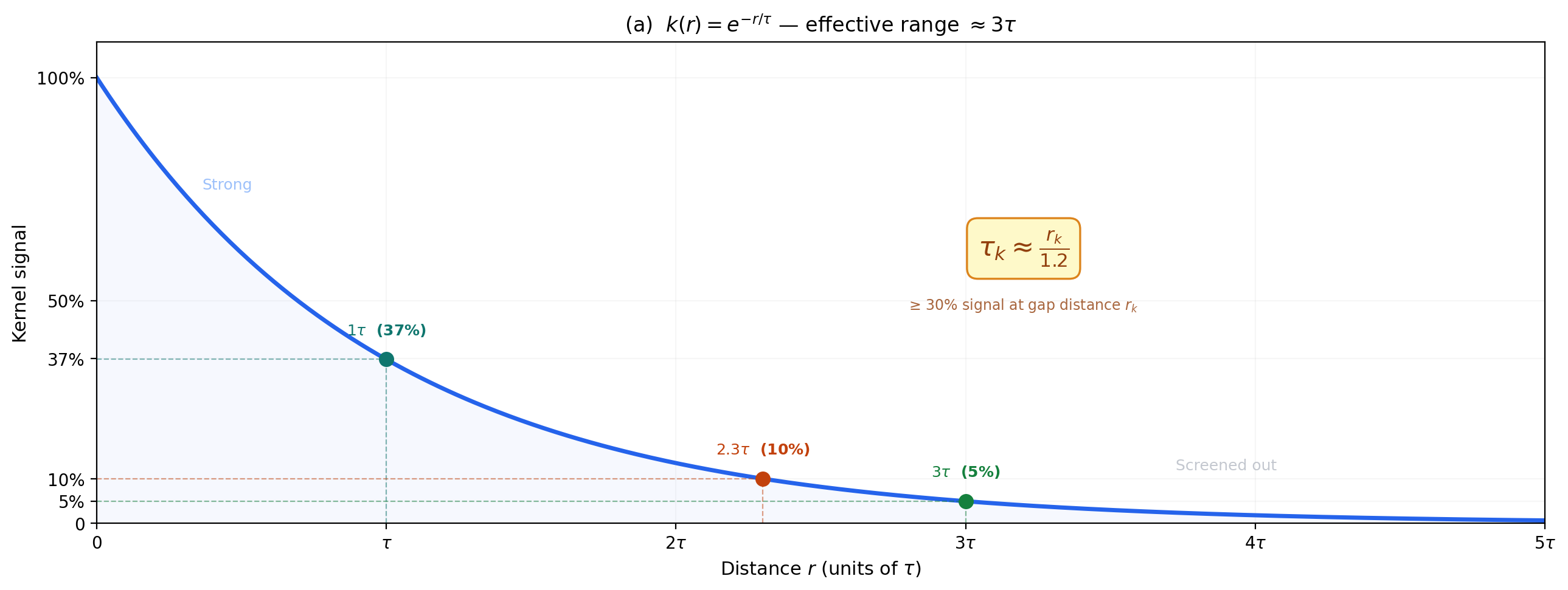
The kernel signal at distance $r$ is:
\[\mathrm{signal}(r) = e^{-r/\tau}\]Setting a threshold:
- At $r = \tau$: signal = $e^{-1} \approx 37\%$
- At $r = 2.3\tau$: signal = $e^{-2.3} \approx 10\%$
- At $r = 3\tau$: signal = $e^{-3} \approx 5\%$
Beyond $\sim 3\tau$, the drift force is effectively zero. A generated point at distance $d \gg 3\tau$ from all data receives no meaningful gradient signal. It is screened out and freezes in place.
This gives a principled design rule. For a generated point at distance $d$ from the nearest data to receive at least 30% of peak signal ($e^{-1.2} \approx 0.30$):
\[\boxed{\tau_k \approx \frac{r_k}{1.2}}\]where $r_k$ is the $k$-th spatial scale you want $\tau_k$ to cover. You need at least one $\tau$ per decade of spatial scale, plus one large $\tau$ to bridge the prior-to-data gap. Without the bridging temperature, the theorem still guarantees the equilibrium exists, but Yukawa screening makes it unreachable from a distant initialization.
The Complete Picture
Theorem (complete). Let $k$ be a strictly positive definite translation-invariant kernel (Laplace, Gaussian, or Matérn) with $k(z) > 0$ and $k(z) \to 0$ as $\lvert z \rvert \to \infty$. For compactly supported probability distributions $p$, $q$:
\[\mathbf{V}_{p,q}(x) = 0 \; \forall x \quad \Longleftrightarrow \quad p = q \tag{13}\]The $(\Leftarrow)$ direction is the paper’s Proposition 3.1 (anti-symmetry). The $(\Rightarrow)$ direction follows from the asymptotic factorization of $\mathcal{K}\lbrack\nu\rbrack(x)$ at large $\lvert x \rvert$: the vanishing drift forces the bilateral Laplace transforms of $p$ and $q$ to have identical log-gradients, which combined with the normalization constraint $\int dp = \int dq = 1$ implies $p = q$.
Practical corollaries:
- Non-SPD kernels (linear, compact, inverse-offset) can fail catastrophically even when training loss converges to zero.
- The paper’s choice of the Laplace kernel is not arbitrary. It is the SPD property that makes the training objective well-founded.
- Choose $\tau_k \approx r_k / 1.2$ where $r_k$ is the $k$-th gap distance in the data, with at least one $\tau$ large enough to reach from the prior to the outermost data structure.
Experimental validation of these predictions for SPD vs non-SPD kernels, compact vs infinite support, single vs multi-temperature schedules, will appear in [Part 2].
References
- Deng, M., Li, H., Li, T., Du, Y., He, K. (2026). Generative Modeling via Drifting. arXiv:2602.04770
- Liu, Z. (2026). On the physical interpretation of drifting generative models. Blog post
- Bochner, S. (1933). Monotone Funktionen, Stieltjessche Integrale und harmonische Analyse. Math. Ann. 108, 378–410
- Wendland, H. (2004). Scattered Data Approximation, Chapter 6. Cambridge University Press.
- Wendland, H. (1995). Piecewise polynomial, positive definite and compactly supported radial functions of minimal degree. Adv. Comput. Math. 4, 389–396
- Sriperumbudur, B. K., Gretton, A., Fukumizu, K., Schölkopf, B., Lanckriet, G. R. G. (2010). Hilbert space embeddings and metrics on probability measures. JMLR 11, 1517–1561
- Gretton, A. et al. (2012). A kernel two-sample test. JMLR 13, 723–773
Citation
If you find this work useful, please cite:
@article{levonyan2026drfitingSPDproof,
  title={Why the Drift Field Finds the Right Distribution: A Bochner Proof},
  author={Levonyan, Karine},
  journal={Blog post},
  year={2026},
  url={https://karinelevonyan.github.io/blog/2026/why-the-drift-field-finds-the-right-distribution-a-bochner-proof-part-1-theory/}
}