Solving the BlueDot Puzzle #1: XOR Geometry, DAS, and a Ring in the Velocity
Below is a write-up of my solution to BlueDot’s TAIS Puzzle #1. The puzzle gave you a five-layer MLP on top of frozen MiniLM embeddings, predicting eight binary features. Seven features are linearly recoverable at layer h2, but one isn’t. The task was to find it, describe the geometry, and then engineer something weirder.
The emphasis is on two parts we found most interesting: establishing causal proof via Distributed Alignment Search (DAS), and a blueprint for constructing hidden, slice-proof representation geometries, what we called a velocity ring.
Key Findings
- Found the hidden feature
country, which collapses to random chance ($0.43$ accuracy) at layerh2because it is hidden as a pure XOR with food ($\cos=-0.99$ between slices). - Applied causal verification via DAS to isolate a 1-D non-linear subspace at
h2. Activation patching this single coordinate flips downstream model outputs, which proves the geometry is actively causal. - Constructed a novel, continuous, zero-mean ring geometry hidden entirely inside the inter-layer velocity update ($v = h_3 - h_2$), achieving absolute linear blindness ($0.32$ accuracy) and defeating single-feature slicing.
Tasks 1 and 2: The Geometry of the Trap
Standard linear probes see nothing at layer h2 because positive country instances sit directly “inside” negative instances along a single axis.
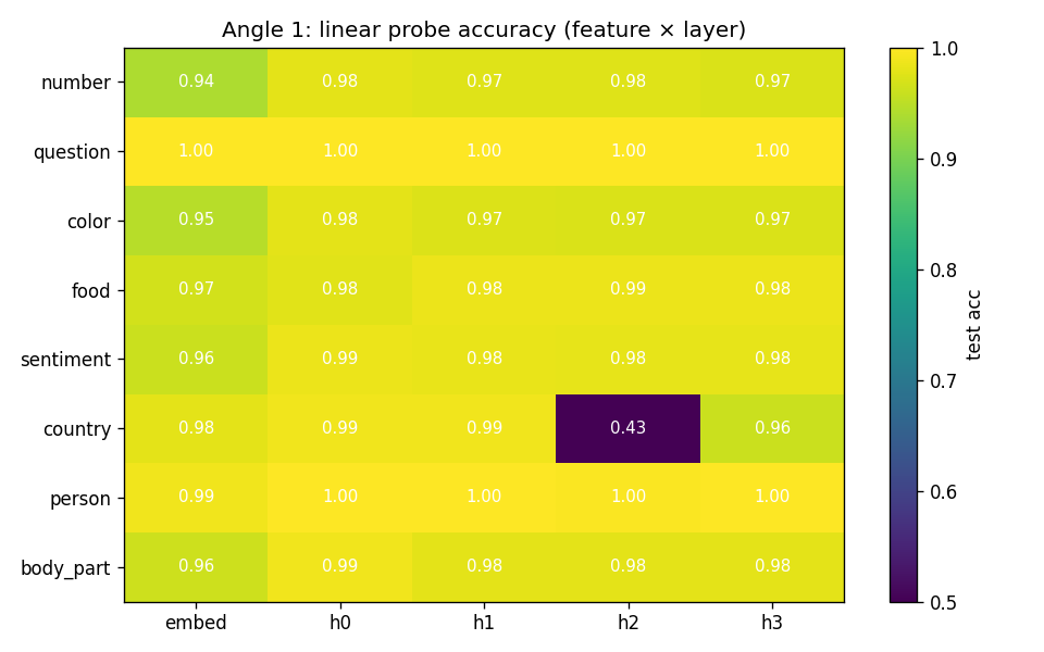
For each layer × feature pair, we fit a linear logistic-regression probe on training activations and score it on test activations. A drop in linear probe accuracy signals a non-linear representation.
| feature | embed | h0 | h1 | h2 | h3 |
|---|---|---|---|---|---|
| number | .94 | .98 | .98 | .98 | .97 |
| question | 1.00 | 1.00 | 1.00 | 1.00 | 1.00 |
| color | .95 | .98 | .97 | .97 | .97 |
| food | .97 | .98 | .99 | .99 | .99 |
| sentiment | .96 | .99 | .98 | .98 | .98 |
| country | .98 | .99 | .99 | .43 | .96 |
| person | .99 | 1.00 | 1.00 | 1.00 | 1.00 |
| body_part | .96 | .99 | .98 | .98 | .98 |
Figure 1. Linear probe accuracy for each feature across layers. Country collapses to 0.43 at h2 and then recovers at h3. Every other feature stays above 0.97 at h2.
Country loses accuracy sharply to 0.43 at h2 and then recovers at h3. A non-linear MLP probe at h2 recovers country to 0.96, so the information is present at h2, just not linearly readable.
No linear probe reads country at h2 because the positive and negative distributions share the same mean. The positive examples sit sandwiched inside the negatives along a single axis:
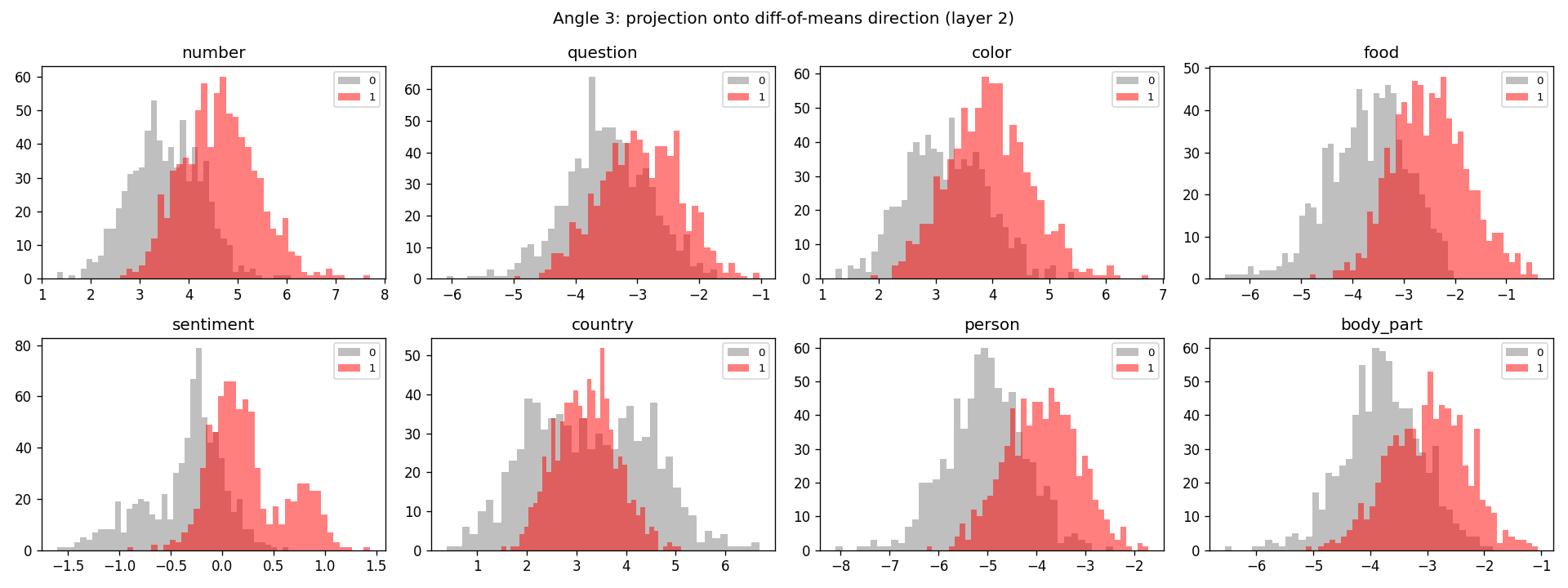 Figure 2. Projection onto each feature’s diff-of-means direction. For country, the red distribution sits inside the gray: no single direction separates them.
The two within-food directions are anti-parallel. A merely food-conditional encoding would force neither. This is the XOR signature, and nothing else produces it. Linear probes fail at h2, but the information is present and causal. We use Distributed Alignment Search (a concept I learned from Atticus Geiger’s lecture at Stanford, from Goodfire.AI) to show that an orthogonal rotation of h2 with interchange interventions on a single rotated coordinate recovers it, and activation patching of that coordinate moves the country output.
| reading of country at h2 | interchange accuracy |
|---|---|
| linear probe | 0.43 |
| random direction | 0.49 |
| linear-probe direction (interchange) | 0.49 |
| learned 1-D DAS subspace | 0.88 |
| full-h2 patch (upper bound) | 0.96 |
We can also project h2 onto the within-food country axis and multiply by the food sign (the XOR-undo). That makes country linearly separable again, lifting probe accuracy from 0.43 to 0.93.
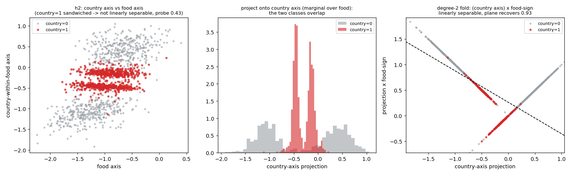 Figure 4. Left: at h2, country=1 (red) is sandwiched inside country=0 (gray), and no line separates them. Middle: marginalising over food, the two classes overlap. Right: the degree-2 fold (projection × food-sign) makes country linearly separable at 0.93. The minimal nonlinearity is a single product with food, exactly the XOR.
Task 3. Weirder Representation
Now for the fun part. We train a weirder representation for the feature F=Sentiment. In this approach the information lives purely in the transition between layers, rather than the state at any single layer. This representation is invisible to standard linear interpretability tools at every step of the computation, yet yields >98% accuracy in the final output.
We encode sentiment with a different, continuous geometry: a zero-mean ring read by its radius. We place it in the velocity: the inter-layer update $v = h_3 - h_2$. To keep the rest of the network identical to the original, we keep the full puzzle head (l1…l5) at full depth for the other seven features and host the ring in a reserved 2-D sub-space of the real update that the readout for the others never touches. In that sub-space the feature is linearly invisible and no single-feature slice unfolds it. Only the radius decodes it.
The full 64-d update still carries sentiment linearly, since the trunk must compute it to build the ring. So the claim is about the readout geometry of the reserved channel, not global linear absence.
The idea is to write the update between hidden layers 2 and 3 as a velocity $v = h_3 - h_2$. We force sentiment to be carried only by the geometry of this update in two reserved dimensions: we push positive examples onto a circle of radius one, negatives sit at the origin, and we make the positives’ angle independent of every label so they cover the whole circle. The result is a ring whose mean is zero, so no linear probe and no PCA direction separates the classes in that sub-space, yet whose radius cleanly decodes sentiment. Because separation needs the radius (a non-linear scalar), conditioning on any other single feature cannot unfold it.
The head is the original puzzle MLP kept at full depth: a frozen all-MiniLM-L6-v2 encoder (mean-pooled 384-dim $x$) feeds l1…l5 exactly as in the puzzle. Three surgical changes, all confined to how sentiment is read and how its channel is reserved:
- Sentiment is read only from the squared radius $v_0^2 + v_1^2$ of the genuine update, never linearly.
l5is masked to zero on the two reserved dims for every output, so the seven regular features, which run the full original depthh2→l4→h3→l5, never read them.- We do not claim the full 64-d update is linearly blind: only the reserved sub-space is.
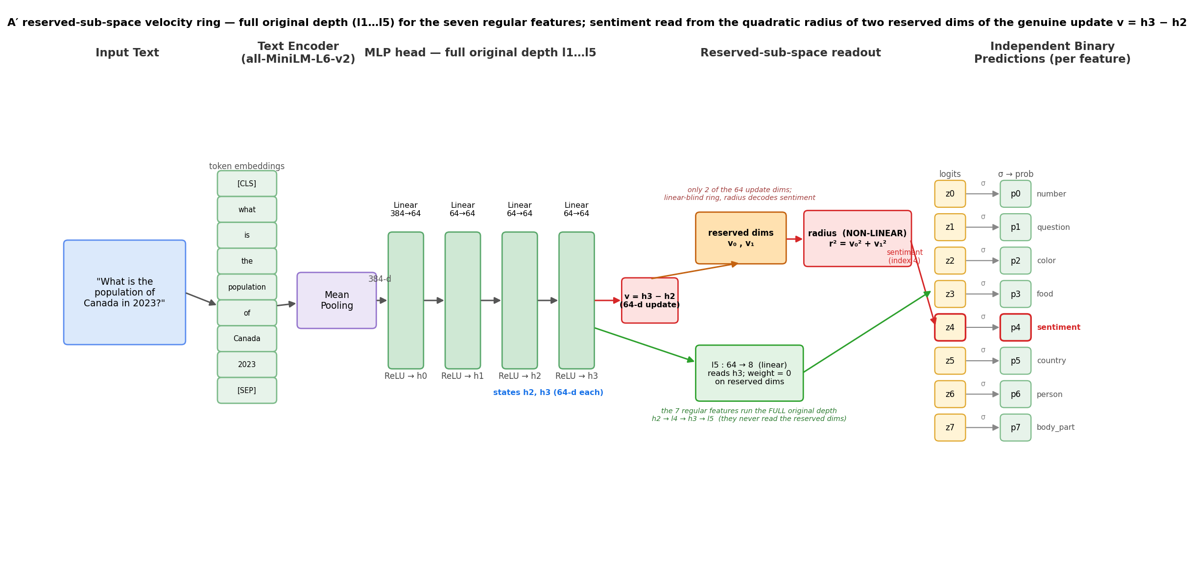 Figure 5. The full head
 l1…l5 is retained: the seven regular features run the original depth h2 → l4 → h3 → l5 (green). We form the genuine inter-layer update v = h3 − h2 (red) and reserve two of its 64 dimensions (orange); l5’s weights are zeroed on those two dims so no other feature reads them. Sentiment is read from the squared radius $r^2 = v_0^2 + v_1^2$ of the reserved dims.
Training uses Adam (lr 1e-3), batch 128, 160 epochs, seed 0, MiniLM frozen. Per batch:
\[L = 10 \cdot L_{\text{BCE}} + 8 \cdot L_{\text{ring}} + 2 \cdot L_{\text{decor}}\]- $L_{\text{BCE}}$: per-feature binary cross-entropy over all eight sigmoid outputs. The model must actually classify every feature, so it must solve sentiment through the radius readout.
- $L_{\text{ring}}$: places the update on the reserved dims $v_r = v[\text{RI}, \text{RJ}]$: for a positive example $|v_r - t_i|^2$ (pull onto the unit circle at a per-example target point $t_i$); for a negative $|v_r|^2$ (pull to the origin).
- $L_{\text{decor}}$: among positives, match the mean of $v_r$ across each other feature’s two values: $\sum_f |\mathbb{E}[v_r \mid f=1] - \mathbb{E}[v_r \mid f=0]|^2$. A belt-and-suspenders term that removes any residual angle–feature correlation.
The hidden part is how the target angle $t_i$ is chosen. This is what makes the ring both linearly blind and slice-proof:
- Draw one fixed random vector $r \in \mathbb{R}^{384}$.
- Orthogonalise $r$ against all eight feature directions. Fit a logistic probe per feature on the embeddings, stack their weight vectors, take an orthonormal basis $Q$ of that span, and remove the component: $r \leftarrow r - Q(Q^\top r)$. Now $r$ is linearly uncorrelated with every label.
- Project every example: $s_i = x_i \cdot r$, then rank-transform $s$ to uniform $u_i \in [0, 1)$. The target angle is $\theta_i = 2\pi u_i$ and $t_i = (\cos\theta_i, \sin\theta_i)$.
The rank makes the angles uniform on the circle, so positives spread evenly and the ring’s mean is ≈ 0. A classifier can only separate two clouds along a direction where their means differ, so a zero-mean ring has no separating hyperplane. The orthogonalisation makes the angle linearly independent of every feature, so within any single-feature slice the positives still cover the whole circle. No 2-feature interaction localises them, which is exactly what defeats slicing.
Why each design choice is necessary
Each ingredient removes a specific, concrete failure mode that appeared when it was absent:
| choice | failure it prevents |
|---|---|
| reserve two dims and mask l5 on them | If l5 were allowed to read the ring dims, the ring would have to share those dimensions with the seven regular features’ readout, exactly the shared-state wall of §3.6, where the linear shadow never leaves. |
| keep full depth l1…l5 for the others | The seven regular features run the original h2 → l4 → h3 → l5 at full depth. Ablating l4 collapses them to chance (§3.6). Their readout is masked off the reserved dims, so the ring losses never trade off against them. |
| radius (quadratic) readout | A linear sentiment head lets the model keep an ordinary linear direction and ignore the ring. Forcing the logit through $v_0^2 + v_1^2$ makes a zero-mean ring the natural and only way to be accurate. |
| rank-uniform, feature-orthogonal angle | With a free angle, the model still made a ring, but tied its angle to another feature; that feature’s slice then unfolded sentiment. Rank-uniform and orthogonalised angles drive every single-feature slice-cell on the reserved dims to ≈0.3. |
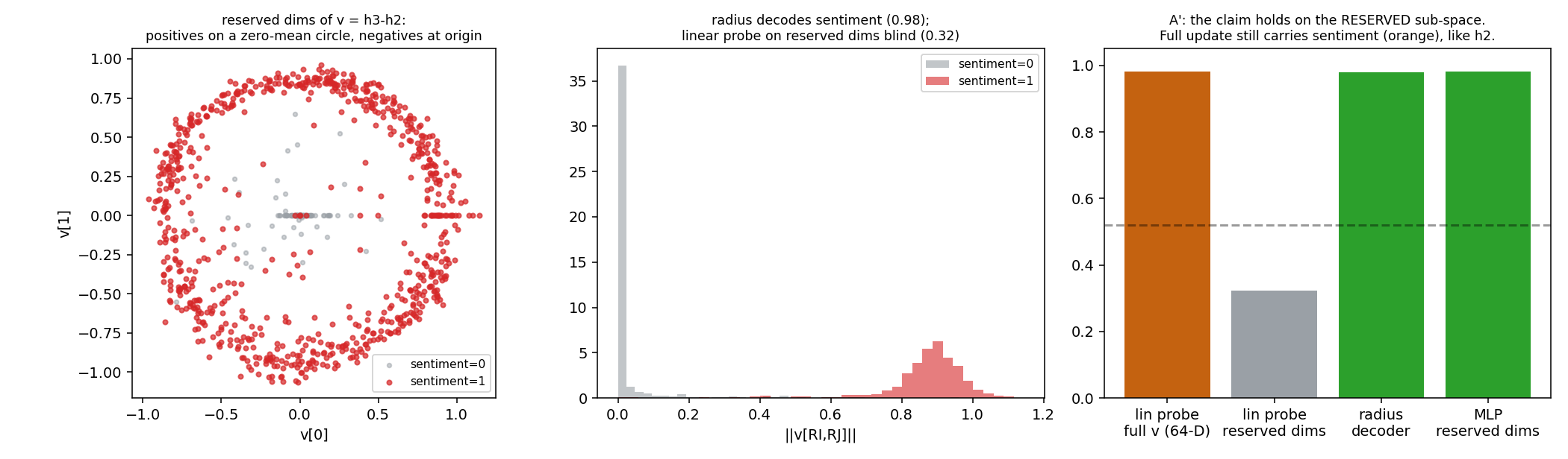
Figure 6. The reserved dims of the genuine update $v = h_3 - h_2$: positive examples (red) lie on a zero-mean circle (radius ≈ 0.87), negatives (gray) at the origin (radius ≈ 0.02). The radius separates the classes cleanly while a linear probe on the reserved dims is at chance.
| quantity | value |
|---|---|
| model accuracy — sentiment (via the ring) | 0.98 |
| model accuracy — all 7 other features | 0.97–1.00 |
| linear probe on reserved dims of the update | 0.32 (chance 0.52) |
| linear probe on full 64-d update $v = h_3 - h_2$ | 0.98 (not blind, honest scope) |
| linear probe on state h2 / h3 | 0.99 / 0.98 |
| radius decoder $\sqrt{v_0^2 + v_1^2}$ on reserved dims | 0.98 |
| defeats single-feature slicing (reserved dims)? | yes, every slice-cell 0.29–0.45 |
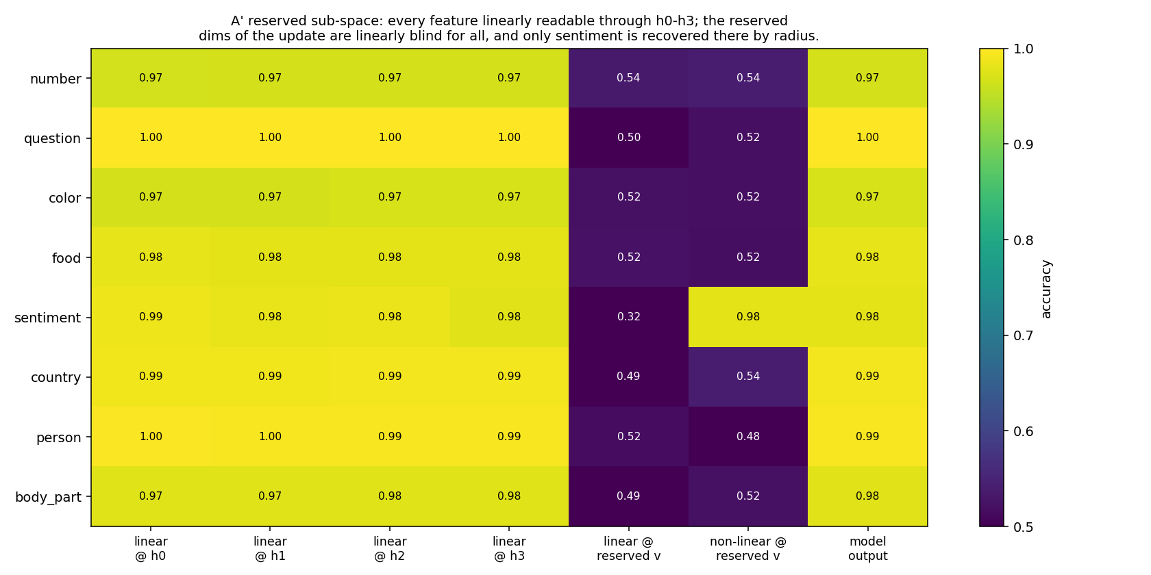
Figure 7. Linear-probe accuracy by feature and channel. The reserved dims of the update are linearly blind for all features; sentiment is only recovered there non-linearly (by its radius).
Training converged the readout to $\text{sentiment} = 9.62 \cdot (v_0^2 + v_1^2) - 3.63$, a circular decision boundary at radius $r^* = 0.61$. Positives land at radius ≈ 0.87 (std 0.13), negatives at ≈ 0.02 (std 0.09); the positive cloud is zero-mean (mean $(+0.05, -0.02)$) and covers the whole circle. The reserved sub-space is genuinely dedicated: a linear probe off the two reserved dims of h3 reads sentiment at 0.97 and every other feature at 0.50–0.54 (chance), and l5’s effective weight on those dims is exactly 0.
We also tried the same trick in a shared state buildig the ring representation but without the velocity concept, but it failed. And that is the same reason why we couldn’t reconstruct the puzzle: a feature that a state must share with the others gets encoded redundantly across its dimensions, so mean-matching leaves a detectable residual, and pushing harder with an adversary destroys the whole state. The reserved-sub-space velocity ring escapes this because the two ring dims are reserved.
Task 4. Reverse Engineering and Why We Failed
We tried to reproduce the puzzle’s XOR encoding by training a model and couldn’t. Retraining the same architecture 147 times across different widths, seeds, and training lengths never produced the collapse: country at h2 stayed ≥0.98 every time, so someone clearly engineered the structure rather than letting it fall out of normal optimization.
We then tried to reconstruct it by penalizing the linear signal at h2 with adversarial probes, alignment losses, and weight surgery. Every attempt hit the same dead end: either the linear shadow simply reformed, or country accuracy collapsed entirely. DAS interchange accuracy was the key diagnostic here. It’s the only metric that distinguishes “information hidden” from “information destroyed,” and it showed there was no middle ground. The puzzle behaves as though the XOR was baked in from the start through direct supervision of the geometry, not patched in afterward. Curious if the puzzle authors would reveal it!
Citation
@article{levonyan2026bluedot,
  title={BlueDot Puzzle #1 Solution},
  author={Levonyan, Karine},
  year={2026},
  url={https://karinelevonyan.github.io/blog/2026/bluedot-puzzle-1/}
}